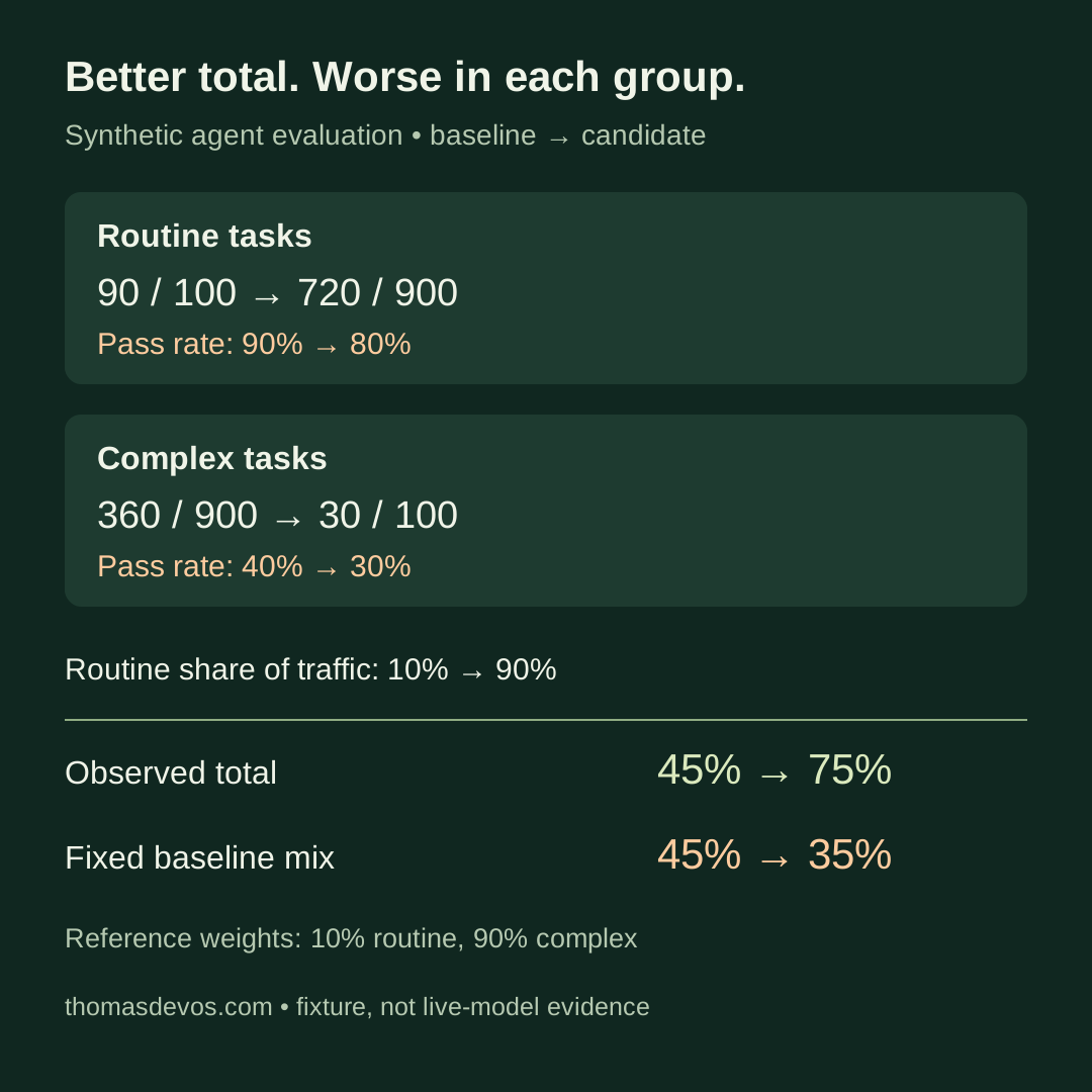
Your agent’s pass rate rises from 45% to 75%. The release dashboard looks reassuring. But routine tasks have fallen from 90% to 80%, and complex tasks from 40% to 30%.
The arithmetic can be correct. The candidate handled far more routine tasks, where its pass rate was higher. That shift outweighed the deterioration inside both groups.
I would require a fixed-reference comparison before accepting an aggregate production score as evidence that an agent improved. The observed score still describes the requests in that period. It cannot, by itself, separate a better implementation from an easier workload.
The counts below are deliberately constructed. This is an executable demonstration of a traffic-mix reversal, not a measured model comparison or a report about a deployed service.
Reproduce the reversal
Imagine two periods of a support-agent service. Each contains 1,000 assessed requests. The grader and the meaning of a pass stay unchanged: the request satisfies its task-specific rubric. For this fixture every request has an observed verdict, and the two groups are mutually exclusive and exhaustive.
| Task group | Baseline passes / requests | Candidate passes / requests |
|---|---|---|
| Routine | 90 / 100 | 720 / 900 |
| Complex | 360 / 900 | 30 / 100 |
| Total | 450 / 1,000 | 750 / 1,000 |
The baseline receives mostly complex requests. The candidate receives mostly routine requests. Within each group, the candidate loses ten percentage points. Across all requests, it gains thirty percentage points.
This is a Simpson’s-paradox-style reversal caused by changing group weights. It differs from the earlier release-gate example where one slice regressed while another improved. That example held the case mix fixed. Here both groups deteriorate, and the changing mix reverses the aggregate direction.
Google’s guidance on evaluating for bias warns that aggregate performance can conceal poor performance on subsets. Its subject is fairness across demographic groups. The task-group example here applies the accounting lesson to operational evaluation; it does not establish a fairness result or replace demographic analysis.
Download agent-eval-traffic-mix.py, inspect it, then run:
python3 agent-eval-traffic-mix.py
python3 agent-eval-traffic-mix.py --test
python3 -O agent-eval-traffic-mix.py --test
The script uses the Python standard library and exact rational arithmetic. It makes no API requests and runs no model. Its demonstration prints:
baseline: observed=45.0%, reference_mix=45.0%
  routine: 90/100 = 90.0%
  complex: 360/900 = 40.0%
candidate: observed=75.0%, reference_mix=35.0%
  routine: 720/900 = 80.0%
  complex: 30/100 = 30.0%
Ten unit tests pass in both ordinary and optimised Python. They check the reversal, the per-group regressions, fixed and equal weighting, order independence, and invalid or missing inputs. Those are ten distinct tests executed twice, not twenty model trials. The script’s successful exit means its own tests passed; it is not a release authorisation for the candidate.
Hold the reference workload fixed
For task group g, let r_g be its pass rate and w_g its share of the workload. The observed aggregate is:
observed pass rate = sum(observed_weight_g * pass_rate_g)
The baseline uses weights of 0.1 for routine and 0.9 for complex. The candidate uses 0.9 and 0.1. Comparing those totals changes both the rates and the weights at once.
A standardised score applies the same declared reference weights to both periods:
reference score = sum(reference_weight_g * pass_rate_g)

baseline:  0.1 * 0.9 + 0.9 * 0.4 = 0.45
candidate: 0.1 * 0.8 + 0.9 * 0.3 = 0.35
At the baseline workload mix, the candidate’s score is 35%, compared with 45% for the baseline. This is an arithmetic reweighting of the observed group rates. It does not prove that replaying the candidate on the old requests would yield exactly 35%.
Equal weights answer another question. Giving each group half the score produces 65% for the baseline and 55% for the candidate. That comparison is useful when the evaluation owner deliberately wants equal group importance. It does not describe either period’s observed traffic.
Do not call this balanced_accuracy_score merely because the weights are equal. Scikit-learn defines balanced accuracy as the average recall across the true classes of a classification problem. These task groups are metadata attached to agent requests, not the classifier’s true labels. The fixture computes weighted task pass rates directly. It borrows no library metric name that would misdescribe the denominator.
Select the reference distribution before examining candidate results. A baseline month, an agreed target workload or a versioned evaluation portfolio can each be defensible. Record the choice and its purpose. Reweighting after seeing the score can become another way to select the answer you wanted.
Keep the observed score beside the reference score
The candidate really did pass 750 of its 1,000 assessed requests. Suppressing that total would discard useful service information. An operations team needs to know the volume and outcomes it actually handled.
A comparison report should retain both views:
- The observed pass rate and request counts for the period.
- Each group’s pass count, denominator and rate.
- The score under a named reference distribution, with those weights visible.
- The required safety checks and their separate release decisions.
In this fixture, the observed total rises while the reference score falls. That is a reason to inspect the workload shift before announcing an improvement. A routing change, a customer rollout or a change in which requests receive labels can all change the mix. None is established by these synthetic counts.
Keep the grouping rule outside the candidate’s control. If the candidate can relabel failed complex tasks as unsupported requests, a fixed weight file will not make the comparison reliable. Preserve the original task label and record any mapping changes as a new evaluation definition.
The downloadable code requires exactly the reference group inventory. A missing group or zero denominator raises an error. It does not renormalise the remaining groups to 100%, which would silently change the target workload. Extra groups also require a deliberate reference update rather than disappearing from the calculation.
Reweighting cannot repair weak observations
A broad group can conceal another mix shift. The candidate’s complex requests might be easier than the baseline’s complex requests, or vice versa. Holding two coarse weights fixed does not make the requests within each group comparable.
For release evaluation, run both implementations on the same versioned case set where feasible. Preserve case-level outcomes so you can inspect paired regressions rather than compare only totals. Reset task state between runs and retain the grader version. If the model is stochastic, decide how repeated trials enter the analysis before collecting them.
For live-service monitoring, report uncertainty and sampling limits. The candidate’s complex group contains only 100 observations in this demonstration. Its observed rate is an input to the arithmetic, not a known population probability. A real comparison needs an uncertainty method appropriate to the sampling process, including clustering when several requests come from one user or workflow. This fixture calculates no confidence intervals and supports no causal claim that a particular release caused the decline.
Missing labels need their own accounting. If difficult requests take longer to assess, today’s apparently easy workload may partly reflect delayed grading. Compare complete windows or report assessed coverage against the full request inventory. Do not silently treat ungraded cases as passes, failures or ordinary exclusions. The article on timeouts and latency denominators examines a related reporting defect: removing unfinished requests can make the observed service look faster.
Reference weights also do not express the cost of an error. A rare unauthorised write may require a blocking gate even if its workload share is tiny. Keep that gate separate from the representative quality score. Choosing a larger weight for permission failures still permits other successes to compensate for them unless the release rule explicitly forbids it.
Add the reference definition to the release record
A small application-owned record is enough to make the comparison inspectable:
{
  "reference_id": "support_mix_fixture_v1",
  "grouping_rule": "task_type_v1",
  "weights": {"routine": "1/10", "complex": "9/10"},
  "missing_group_policy": "comparison_unavailable",
  "grader_version": "fixture_boolean_v1"
}
This is illustrative metadata, not a vendor setting. The script defines the weights directly as Fraction values; it does not load this JSON. A production loader would need to validate the inventory and parse those rational strings, as well as bind the record to the actual case and result files.
For the broader work of building graders and release evidence, my book AI Agent Evals on Leanpub covers evaluation harnesses and practical labs. This fixture is a separate, focused accounting example.
Add a fixed-reference score beside the observed total in your next comparison. If the two move in opposite directions, inspect the group counts before attributing the change to the agent.