A dashboard that averages worker p95 values can report a service latency that none of its users experienced. Weighting those percentiles by request count does not repair the calculation.
For an agent service, that error can affect routing decisions, capacity plans and release gates. A team may think a model change meets its latency target because the dashboard combined already-compressed summaries instead of the underlying request distribution.
I would reject a service-level p95 panel whose query averages per-worker quantiles. Keep observations in a form that can be merged, then calculate the percentile over the population the panel claims to describe.
Reproduce the error before changing the dashboard
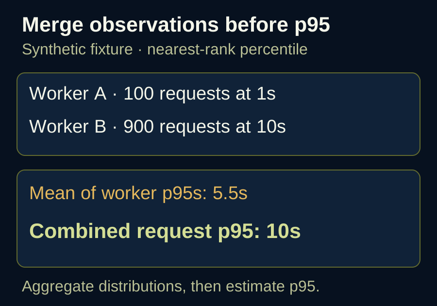
Use a synthetic workload with deliberately simple timings. Worker A completes 100 requests, all in one second. Worker B completes 900 requests, all in ten seconds. The fixture uses the nearest-rank definition of a percentile: sort the observations and select the value at rank ceil(p × n), counting ranks from one.
| Calculation | Result |
|---|---|
| Worker A p95 | 1 second |
| Worker B p95 | 10 seconds |
| Unweighted mean of worker p95s | 5.5 seconds |
| Request-weighted mean of worker p95s | 9.1 seconds |
| p95 of all 1,000 requests | 10 seconds |
The combined distribution contains 100 one-second requests followed by 900 ten-second requests. Its 950th observation is ten seconds. Neither average recovers that value.
Other percentile conventions interpolate between observations. The chosen convention should be documented, especially for small samples. It does not make averaging independently computed quantiles a valid way to reconstruct the pooled distribution.
The downloadable fixture calculates all five results and checks them with assertions. Run it with Python 3; it has no external dependencies.
from math import ceil


def nearest_rank(values, p):
    if not values or not 0 < p <= 1:
        raise ValueError("require observations and 0 < p <= 1")
    ordered = sorted(values)
    return ordered[ceil(p * len(ordered)) - 1]


a = [1.0] * 100
b = [10.0] * 900
assert nearest_rank(a + b, 0.95) == 10.0
This is an arithmetic counterexample, not a benchmark of any model provider. Real workloads contain a wider distribution of durations, errors and request lengths. That adds reasons to retain distribution information.
Aggregate histogram buckets before estimating p95
Prometheus documents the distinction between histograms and summaries: histograms retain an aggregatable representation of observations, while a summary’s precomputed quantiles cannot be aggregated into a service quantile.
For a classic histogram named agent_request_duration_seconds, the following query estimates p95 across instances for each route over a five-minute window:
histogram_quantile(
  0.95,
  sum by (le, route) (
    rate(agent_request_duration_seconds_bucket[5m])
  )
)
This example assumes the selected series describe the same request boundary and use compatible bucket boundaries. In a shared monitoring system, add selectors for the intended service and environment. The route label should be a bounded service route, never a raw prompt or request identifier.
Apply rate to each original series before summing so counter resets can be handled at the series level. Preserve le, the classic histogram bucket boundary label, during aggregation. The query then estimates a percentile from the aggregated buckets rather than averaging percentiles calculated elsewhere.
Bucket resolution limits the estimate. If the latency objective falls inside a wide bucket, the interpolated p95 may not resolve a small regression reliably. Choose boundaries around the operational thresholds you need to inspect, or use supported native histograms with appropriate resolution. Native histograms use a different query shape; do not copy the classic _bucket query into a native-histogram panel unchanged.
A panel also needs an observation count. Sparse traffic and a short window can produce unstable tail estimates. A smooth line alone does not tell the reviewer how many requests support it.
Decide when an agent request starts and ends
For a tool-using agent, a provider-call histogram and a user-request histogram measure different operations. A user request may include retrieval, several model calls, tool execution and retries. Summing the p95 of each component does not yield the p95 of total elapsed request time. Parallel work makes that interpretation even less defensible.
Instrument elapsed time at the user-request boundary if the objective concerns the user’s wait. Keep component durations for diagnosis. Use a monotonic clock within the measuring process so wall-clock corrections do not distort elapsed duration.
Streaming adds another boundary. Time to first visible content can improve while time to a complete usable answer worsens. Name both metrics explicitly. If a streamed answer can later fail verification, first content is not evidence that the request completed successfully.
Record terminal outcomes alongside duration: success, timeout, cancellation and failure. A success-only histogram answers how long successful requests took. It cannot describe the experience of every arrival. For a timeout, record the observed time until termination; the duration a successful completion would have required remains unknown.
Test the panel with an uneven traffic split
A routing change can move traffic between workers without changing either worker’s latency distribution. Keep the synthetic unequal-volume fixture as a regression check for dashboard logic. An average of worker percentiles will fail it even though every individual worker panel is correct.
When reviewing a release, inspect the query, metric boundary, terminal outcomes, bucket configuration and observation count. Save those definitions with the latency result. The next person investigating a slow agent needs to know whether the reported p95 covers complete user requests, successful model calls or the first fragment of streamed text.